ClearSCADA can perform calculations on the raw historic values in your database (see Raw Historic Data on Trends). The results of these calculations are called processed historic data, and like raw historic values, they can be used as the data source for a trace on a Trend.
The main benefits of processed historic data are:
- You can use processed historic data to view statistical information on a Trend. For example, you can use historic algorithms to set a trace to represent the average values of a data source. With raw historic data, you can only view the actual values that are stored historically in the database.
There are many different types of algorithm (calculation) that you can use to produce processed historic data (see Built-In Historic Algorithms for Processed Historic Data).
- You can control how many historic values are plotted on a Trend.
If your Trend is configured to show a raw historic trace, the trace has to plot each of the historic values for the time shown on the X-axis. So, if the X-axis is set to represent 1 day and the data source of the trace has historic values for every second, the trace will have to plot 86, 400 values. Plotting each of the raw historic values can result in a cluttered Trend that is difficult to use (although ClearSCADA does have built-in mechanisms to stop Trends from drawing an excessive amount of values and markers, see Summary Mode for Processed Historic Traces).
With processed historic data, you have greater control over the amount of values that are shown on a trace as you can set the resample interval (see Resample Interval for Processed Historic Data). The resample interval is a time period that defines when a historic value is calculated. For example, if you define a resample interval of 5M, it means ClearSCADA will calculate a new processed historic value every 5 minutes. So, for the processed historic value for 11:05, ClearSCADA would perform the calculation using the raw historic values for the period 11:00-11:05. The result of the calculation is the processed historic value that is drawn on the trace for 11:05. The next processed historic value is drawn at 11:10. This means that there are fewer values and markers on the trace.
Take care with End and End Last Historic Algorithms used on clients, or with ClearSCADA features, that run in Local Time with Daylight Saving Time. Ensure that the start and end times specified for the sample interval do not coincide exactly with the time at which the clock jumps backward. Include a small offset in the sample time, to offset the calculation to avoid the sample end or start time exactly matching the time that the clock jumps backward at the transition from Daylight Saving Time to Standard Time. A small offset of 1s or even 1ms should suffice. For more information about Daylight Saving Time, see The Effects of Daylight Saving Time Adjustments.
Example:
A point is used to monitor the flow of water in a pipe and it is set to update every second. The point has the historic feature enabled and so a raw historic value is stored for the point each second.
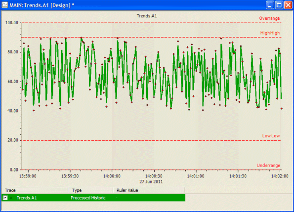
An engineer wants to view the point’s values over the period of an entire hour and so creates a Trend with an X-axis set to represent 1 hour. The engineer then adds a trace to represent the point’s raw historic values. As the engineer knows the point has 3600 values for the required period, they alter the markers setting of the trace to 3600 so that a marker can be drawn for each value.

The trace is drawn, but is difficult to read because of the high density of values on show.

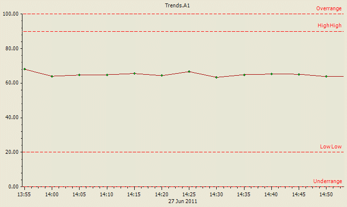
To make the Trend easier to use, the engineer creates a new trace; a processed historic trace for the same point. The trace is configured so that it uses the Average algorithm and has a resample interval of 5M (five minutes). This means that ClearSCADA will calculate the average value of the point and plot the result on the trace in five minute intervals. To calculate the average value, ClearSCADA will use the raw historic values for each 5 minute interval.
To make the Trend easier to use, the engineer uses the Show>None feature for the raw historic trace so that only the processed historic trace is visible.

The processed historic trace provides the engineer with the average values of the point over the 1 hour period. There are fewer values and markers as the processed historic values are calculated at 5 minute intervals (as defined by the resample interval) rather than every second. This allows the engineer to see rises and drops in the point’s value over the hour without the need to view the large number of raw historic values.